Running experiments on a cluster

For many research projects in quantum error correction, running experiments on a computer cluster is needed to produce convincing results on large code distances. PanQEC contains an extensive set of tools to help you run experiments on a cluster painlessly. It includes commands to run experiments in parallel on a given number of cores, to generate scripts for Slurm, SGE and PBS cluster management systems, to automatically save experiments in real-time, and to check the progress of your experiments at any point.

In this tutorial, we will cover the whole pipeline of a cluster experiment, from creating the input files to plotting the final results on your laptop.

Folder structure

In this tutorial, we will adopt the following folder structure for the experiment:

my-experiment/: root folder that will contain all the data of the experiments
- my-experiment/inputs/: contains the input json file(s)
- my-experiment/results/: contain the result json files (once the experiments is running)
- my-experiment/logs/: contain the log files of the experiment, such as the current progress and the CPU/RAM usage.

The my-experiment folder and the inputs subfolder will be automatically generated with the panqec generate-input command. The subfolders results and logs will be created automatically when starting the experiment.

Creating the input files

PanQEC works by processing input files written in a json format. Those specify most details of the experiments you want to run: the code/decoder/error model to use and their parameters, the lattice sizes, the physical error rates, etc. Here is an example of input file that describes a 2D toric code simulation under depolarizing noise, decoded using minimum-weight perfect matching:

{
    "comments": "",
    "ranges": {
        "label": "toric-2d-experiment",
        "method": {
            "name": "direct",
            "parameters": {}
        },
        "code": {
            "name": "Toric2DCode",
            "parameters": [
                {
                    "L_x": 5,
                    "L_y": 5,
                },
                {
                    "L_x": 7,
                    "L_y": 7,
                },
                {
                    "L_x": 9,
                    "L_y": 9,
                }
            ]
        },
        "error_model": {
            "name": "PauliErrorModel",
            "parameters": {
                "r_x": 0.33333333333333337,
                "r_y": 0.33333333333333337,
                "r_z": 0.3333333333333333
            }
        },
        "decoder": {
            "name": "MatchingDecoder",
            "parameters": {}
        },
        "error_rate": [
            0.1,
            0.11,
            0.12,
            0.13,
            0.14,
            0.15,
            0.16,
            0.17,
            0.18,
            0.19,
            0.2,
        ]
    }
}

Let’s analyze the different parts of this input json file:

label is a name you want to give to this experiment
method specifies the simulation method. For the moment, there are two different methods: direct and splitting. The direct method consists in sampling independent errors at each Monte-Carlo round, while the splitting method samples errors using a Monte-Carlo Markov Chain algorithm introduced in this paper by Bravyi and Vargo. The splitting method has not been as thoroughly tested as the direct one in PanQEC at the moment, and we would advise against using it.
code: name and parameters of the code. The list of all codes can be found using the command line panqec ls codes. L_x, L_y (and L_z for 3D codes) define the lattice dimensions.
error_model: name and parameters of the error model. At the moment, there is only one error model called PauliErrorModel, which samples i.i.d Pauli errors at each run, without any measurement error. It is specified by three parameters, (r_x, r_y, r_z), which define the rate of Pauli $X$, $Y$ and $Z$ errors respectively. They should therefore all lie between $0$ and $1$ and satisfy the constraint $r_x+r_y+r_z=1$.
decoder: name and parameters of the decoder. The list of all decoders can be found using the command line panqec ls decoders.
error_rate: list of physical error rates included in the simulation.

The above input file can be generated by using the panqec generate-input command as follows.

panqec generate-input -d "my-experiment" \
    --code_class Toric2DCode --sizes "5x5,7x7,9x9" \
    --decoder_class MatchingDecoder \
    --bias "Z" --eta "0.5" \
    --prob "0.1:0.2:0.01"

The above command will create a directory called my-experiment in the current working directory with the file structure previously described. Specifically, the input file will be written to my-experiment/inputs/experiment.json, which you may inspect.

The only non-obvious parameters might be bias and eta. The parameter bias can be either X, Y or Z, and eta can be any value between 0.5 and inf, where eta=0.5 corresponds to depolarizing noise and eta=inf to pure {X,Y,Z} noise (depending on the value of bias). See panqec generate-input --help for more information.

To test that the input file is correct and that all the libraries are correctly installed, we recommand you to do a mock run with the following command:

panqec run -i my-experiment/inputs/experiment.json -o mock.json.gz -t 10

This will run your experiment with 10 trials and store the result in a compressed json file mock.json.gz

Generating cluster script

PanQEC has a command to automatically generate a cluster script, namely panqec generate-cluster-script. Its first input is a header file. It should contain the template for the first few lines a cluster script, which must be tailored for your specific cluster. Here is an example of a header file for Slurm (note that your cluster may require a slightly different format):

#!/bin/bash
#SBATCH -N 1
#SBATCH -t ${TIME}
#SBATCH --cpus-per-task=${N_CORES}
#SBATCH --exclusive
#SBATCH --job-name=${NAME}
#SBATCH --array=1-${N_NODES}
#SBATCH --mem=${MEMORY}
#SBATCH -p ${QUEUE}
#SBATCH --output=${DATA_DIR}/%j.out

module purge
module load gcc/devtoolset/9
module load anaconda/anaconda3.7
source ~/.bashrc

All the variables enclosed by ${} will be replaced by an actual value in generated cluster scripts. Once you have this header ready, let’s say in a file slurm_header.sbatch, you can run the following command:

panqec generate-cluster-script \
       slurm_header.sbatch \
       --output-file my-experiment/run.sbatch \
       --data-dir my-experiment \
       --cluster slurm \
       --trials 10000 \
       --n-nodes 8 \
       --n-cores 5 \
       --wall-time "00:10:00" \
       --memory "1G" \
       --partition debug \
       --delete-existing

You should now have the following content in the generated cluster script my-experiment/run.sbatch:

#!/bin/bash
#SBATCH -N 1
#SBATCH -t 00:10:00
#SBATCH --cpus-per-task=5
#SBATCH --exclusive
#SBATCH --job-name=my-experiment
#SBATCH --array=1-8
#SBATCH --mem=1G
#SBATCH -p debug
#SBATCH --output=my-experiment/%j.out

module purge
module load gcc/devtoolset/9
module load anaconda/anaconda3.7
source ~/.bashrc

panqec monitor-usage my-experiment/logs/usage_$SLURM_JOB_ID_$SLURM_ARRAY_TASK_ID.txt &

panqec run-parallel -d my-experiment -n 8 -j $SLURM_ARRAY_TASK_ID -c 5 -t 10000 --delete-existing

date

As you can see, it first contains a command to monitor the resource usage (CPU and RAM), which will be stored in the logs directory. The second command, run-parallel, parallelizes the 10000 Monte Carlo trials over all the nodes and cores, and runs the simulation on the current node of the job array.

Running the script and checking progress

Simply run the script generated above with your cluster system command to submit jobs. For instance, in Slurm, enter:

sbatch my-experiment/run.sbatch

You can check the progress of the experiment with the command

panqec check-progress my-experiment/logs

The above will display a progress bar shown how much has been completed. You can add the option -a to inspect the progress on all the cores individually

You can also graphically check the usage of available resources using

panqec check-usage my-experiment/

which will plot the RAM and CPU usage over time in the command line.

Aggregating and analyzing results

Once the experiment is running, all the results will be regularly saved in the files my-experiment/results/results_[i].json.gz where [i] is the index of the core. At any moment during the experiment, you can merge the results into a single file and send it to your laptop for analysis. Here is the command you need to run:

panqec merge-results my-experiment/results/results_* -o my-experiments/merged-results.json.gz

You can then send the file my-experiment/merged-results.json.gz to your laptop using scp, rsync or an equivalent method. For example, if my-experiment is in your cluster’s home directory then you can sync it to a local directory called my-experiment/ on your laptop by running the following command on your laptop:

rsync -avzhe ssh user@example.com:~/my-experiments/merged-results.json.gz my-experiment/

Of course, you should replace user and example.com with your appropriate username and cluster URL.

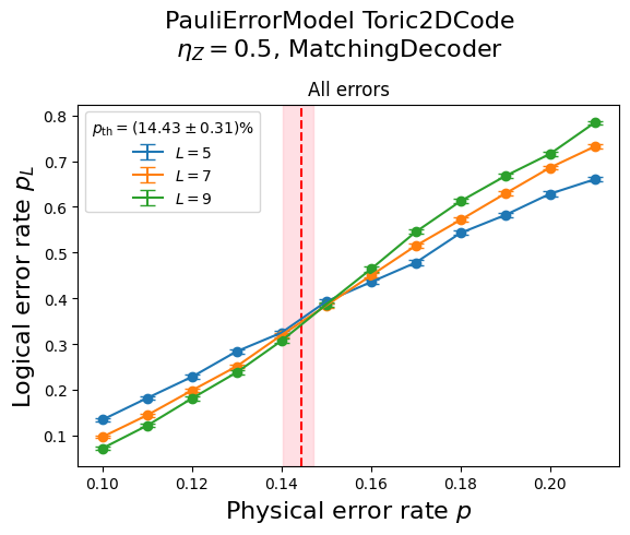
The following piece of code, which you can run locally on a Jupyter Notebook, will allow you to quickly visualize the obtained data and estimate the threshold.

[1]:

from panqec.analysis import Analysis
analysis = Analysis("my-experiment/merged-results.json.gz")
analysis.plot_thresholds()

../_images/tutorials_Running_experiments_on_a_cluster_34_0.png

If you wish to inspect the data yourself, just use the get_results() method. For example,

[3]:

df = analysis.get_results()
df[['code', 'd', 'error_model', 'bias', 'decoder', 'error_rate', 'n_fail', 'n_trials']].head(10)

[3]:

	code	d	error_model	bias	decoder	error_rate	n_fail	n_trials
0	Toric2DCode	5	PauliErrorModel	0.5	MatchingDecoder	0.10	1347	10000
1	Toric2DCode	5	PauliErrorModel	0.5	MatchingDecoder	0.11	1821	10000
2	Toric2DCode	5	PauliErrorModel	0.5	MatchingDecoder	0.12	2284	10000
3	Toric2DCode	5	PauliErrorModel	0.5	MatchingDecoder	0.13	2841	10000
4	Toric2DCode	5	PauliErrorModel	0.5	MatchingDecoder	0.14	3249	10000
5	Toric2DCode	5	PauliErrorModel	0.5	MatchingDecoder	0.15	3931	10000
6	Toric2DCode	5	PauliErrorModel	0.5	MatchingDecoder	0.16	4355	10000
7	Toric2DCode	5	PauliErrorModel	0.5	MatchingDecoder	0.17	4781	10000
8	Toric2DCode	5	PauliErrorModel	0.5	MatchingDecoder	0.18	5428	10000
9	Toric2DCode	5	PauliErrorModel	0.5	MatchingDecoder	0.19	5820	10000

In the above table, error_rate is the physical error rate, n_fail is the number of decoding failures and n_trials is the number of trials simulated.

You can also inspect the numerical values of the threshold estimates.

[4]:

analysis.thresholds[['code', 'error_model', 'bias', 'p_th_fss', 'p_th_fss_left', 'p_th_fss_right']]

[4]:

	code	error_model	bias	p_th_fss	p_th_fss_left	p_th_fss_right
0	Toric2DCode	PauliErrorModel	0.5	0.144347	0.14033	0.147065

In the above table, p_th_fss is the threshold estimate by finite-size scaling and p_th_fss_left and p_th_fss_right are left and right $1\sigma$ CI bounds on the estimate.

More detailed on the Analysis class can be found in the tutorial Computing the Threshold of the Surface Code and in the documentation.